Model fitting
Fitting procedure
SExtractor can fit models to the images of detected objects since version 2.8. The fit is performed by minimizing the loss function
with respect to components of the model parameter vector \(\boldsymbol{q}\). \(\boldsymbol{q}\) comprises parameters describing the shape of the model and the model pixel coordinates \(\boldsymbol{x}\).
Modified least squares
The first term in (1) is a modified weighted sum of squares that aims at minimizing the residuals of the fit. \(p_i\), \(\tilde{m}_i(\boldsymbol{q})\) and \(\sigma_i\) are respectively the pixel value above the background, the value of the resampled model, and the pixel value uncertainty at image pixel \(i\). \(g(u)\) is a derivable monotonous function that reduces the influence of large deviations from the model, such as the contamination by neighbors (Fig. 8):
\(u_0\) sets the level below which \(g(u)\approx u\). In practice, choosing \(u_0 = \kappa \sigma_i\) with \(\kappa = 10\) makes the first term in (1) behave like a traditional weighted sum of squares for residuals close to the noise level.
Caution
The cost function in (1) is optimized for Gaussian noise and makes model-fitting in SExtractor appropriate only for image noise with a pdf symmetrical around the mean.
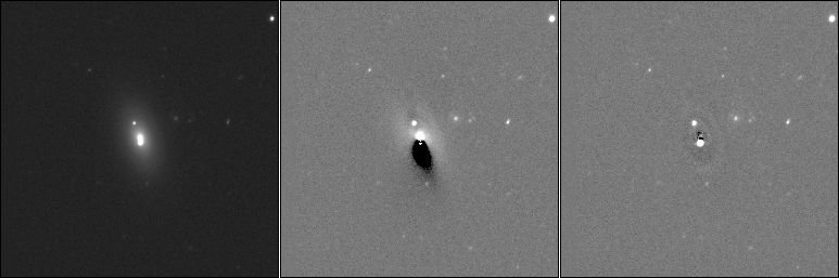
Fig. 8 Effect of the modified least squares loss function on fitting a model to a galaxy with a bright neighbor. Left: the original image; Middle: residuals of the model fitting with a regular least squares (\(\kappa = +\infty\)); Right: modified least squares with \(\kappa = 10\).
The vector \(\tilde{\boldsymbol{m}}(\boldsymbol{q})\) is obtained by convolving the high resolution model \(\boldsymbol{m}(\boldsymbol{q})\) with the local PSF model \(\boldsymbol{\phi}\) and applying a resampling operator \(\mathbf{R}(\boldsymbol{x})\) to generate the final model raster at position \(\boldsymbol{x}\) at the nominal image resolution:
\(\mathbf{R}(\boldsymbol{x})\) depends on the pixel coordinates \(\boldsymbol{x}\) of the model centroid:
where \(h\) is a 2-dimensional interpolant (interpolating function), \(\boldsymbol{x}_i\) is the coordinate vector of image pixel \(i\), \(\boldsymbol{x}_j\) the coordinate vector of model sample \(j\), and \(\eta\) is the image-to-model sampling step ratio (sampling factor) which is by default defined by the PSF model sampling. We adopt a Lánczos-4 function [15] as interpolant.
Change of variables
Many model parameters are valid only over a restricted domain. Fluxes, for instance, cannot be negative. In order to avoid invalid values and also to facilitate convergence, a change of variables is applied individually to each model parameter:
The “model” variable \(q_j\) is bounded by the lower limit \(a_j\) and the upper limit \(b_j\) by construction. The “engine” variable \(Q_j\) can take any value, and is actually the parameter that is being adjusted in the fit, although it does not have any physical meaning. In SExtractor three different types of transforms \(f_j()\) are applied, depending on the parameter (Table 5).
| Type | Model \(\stackrel{f^{-1}}{\to}\) Engine | Engine \(\stackrel{f}{\to}\) Model | Examples |
|---|---|---|---|
| Unbounded (linear) | \(Q_j = q_j\) | \(q_j = Q_j\) | SPHEROID_POSANGLE
DISK_POSANGLE
|
| Bounded linear | \(Q_j = \ln \frac{q_j - a_j}{b_j - q_j}\) | \(q_j = \frac{b_j - a_j}{1 + \exp -Q_j} + a_j\) | XMODEL_IMAGE
SPHEROID_SERSICN
|
| Bounded logarithmic | \(Q_j = \ln \frac{\ln q_j - \ln a_j}{\ln b_j - \ln q_j}\) | \(q_j = a_j \frac{\ln b_j - \ln a_j}{1 + \exp -Q_j}\) | FLUX_SPHEROID
DISK_ASPECT
|
In practice, this approach works well, and was found to be much more reliable than a box constrained algorithm [16].
Regularization
Although minimizing the (modified) weighted sum of least squares gives a solution that fits best the data, it does not necessarily correspond to the most probable solution given what we know about celestial objects. The discrepancy is particularly significant in very faint (SNR \(\le 20\)) and barely resolved galaxies, for which there is a tendency to overestimate the elongation, known as the “noise bias” in the weak-lensing community [17][18][19][20]. To mitigate this issue, SExtractor implements a simple Tikhonov regularization scheme on selected engine parameters, in the form of an additional penalty term in (1). This term acts as a Gaussian prior on the selected engine parameters. However for the associated model parameters, the change of variables can make the (improper) prior far from Gaussian. Currently the only regularized parameter is SPHEROID_ASPECT_IMAGE (and its derivatives SPHEROID_ASPECT_WORLD, ELLIP1MODEL_IMAGE, etc.), for which \(\mu_{\tt SPHEROID\_ASPECT} = 0\) and \(s_{\tt SPHEROID\_ASPECT} = 1\) (Fig. 9).

Fig. 9 Effect of the Gaussian prior on the SPHEROID_ASPECT_IMAGE model parameter. Left: change of variables between the model (in abscissa) and the engine (in ordinate) parameters. Right: equivalent (improper) prior applied to SPHEROID_ASPECT_IMAGE for \(\mu_{\tt SPHEROID\_ASPECT} = 0\) and \(s_{\tt SPHEROID\_ASPECT} = 1\) in equation (1).
Minimization
Minimization of the loss function \(\lambda(\boldsymbol{q})\) is carried out using the Levenberg-Marquardt algorithm, and more specifically the LevMar implementation [21]. The library approximates the Jacobian matrix of the model from finite differences using Broyden’s [22] rank one updates. The fit is done inside a disk which diameter is scaled to include the isophotal footprint of the object, plus the FWHM of the PSF, plus a 20 % margin.
The number of iterations is returned in the NITER_MODEL measurement parameter. It is generally a few tens. The final value of the modified chi square term in (1), divided by the number of degrees of freedom, is returned in CHI2_MODEL.
The FLAGS_MODEL catalog parameter flags various issues which may happen during the fitting process (see the Flagging section for details on how flags are managed in SExtractor):
| Value | Meaning |
|---|---|
| 1 | the unconvolved, supersampled model raster exceeds 512×512 pixels and had to be resized |
| 2 | the convolved, resampled model raster exceeds 512×512 pixels and had to be resized |
| 4 | not enough pixels are available for model fitting on the measurement image (less pixels than fit parameters) |
| 8 | at least one of the fitted parameters hits the lower bound |
| 16 | at least one of the fitted parameters hits the upper bound |
\(1\,\sigma\) error estimates are provided for most measurement parameters; they are obtained from the full covariance matrix of the fit, which is itself computed by inverting the approximate Hessian matrix of \(\lambda(\boldsymbol{q})\) at the solution.
Models
Models contain one or more components, which share their central coordinates. For instance, a galaxy model may be composed of a spheroid (bulge) and a disk components. Both components are concentric but they may have different scales, aspect ratios and position angles. Adding a component is done simply by invoking one of its measurement parameters in the parameter file, e.g., DISK_SCALE_IMAGE.
The present version of SExtractor supports the following models
BACKOFFSET: flat background offset
Relevant measurement parameters: FLUX_BACKOFFSET, FLUXERR_BACKOFFSET
POINT_SOURCE: point source
Relevant measurement parameters: FLUX_POINTSOURCE, FLUXERR_POINTSOURCE, MAG_POINTSOURCE, MAGERR_POINTSOURCE, FLUXRATIO_POINTSOURCE, FLUXRATIOERR_POINTSOURCE
DISK: exponential disk
Relevant measurement parameters: FLUX_DISK, FLUXERR_DISK, MAG_DISK, MAGERR_DISK, FLUXRATIO_DISK, FLUXRATIOERR_DISK, FLUX_MAX_DISK, MU_MAX_DISK, FLUX_EFF_DISK, MU_EFF_DISK, FLUX_MEAN_DISK, MU_MEAN_DISK, DISK_SCALE_IMAGE, DISK_SCALEERR_IMAGE, DISK_SCALE_WORLD, DISK_SCALEERR_WORLD, DISK_ASPECT_IMAGE, DISK_ASPECTERR_IMAGE, DISK_ASPECT_WORLD, DISK_ASPECTERR_WORLD, DISK_INCLINATION, DISK_INCLINATIONERR, DISK_THETA_IMAGE, DISK_THETAERR_IMAGE, DISK_THETA_WORLD, DISK_THETAERR_WORLD, DISK_THETA_SKY, DISK_THETA_J2000, DISK_THETA_B1950
SPHEROID: Sérsic (\(R^{1/n}\)) spheroid
FLUX_SPHEROID, FLUXERR_SPHEROID, MAG_SPHEROID, MAGERR_SPHEROID, FLUXRATIO_SPHEROID, FLUXRATIOERR_SPHEROID, FLUX_MAX_SPHEROID, MU_MAX_SPHEROID, FLUX_EFF_SPHEROID, MU_EFF_SPHEROID, FLUX_MEAN_SPHEROID, MU_MEAN_SPHEROID, SPHEROID_SCALE_IMAGE, SPHEROID_SCALEERR_IMAGE, SPHEROID_SCALE_WORLD, SPHEROID_SCALEERR_WORLD, SPHEROID_ASPECT_IMAGE, SPHEROID_ASPECTERR_IMAGE, SPHEROID_ASPECT_WORLD, SPHEROID_ASPECTERR_WORLD, SPHEROID_INCLINATION, SPHEROID_INCLINATIONERR, SPHEROID_THETA_IMAGE, SPHEROID_THETAERR_IMAGE, SPHEROID_THETA_WORLD, SPHEROID_THETAERR_WORLD, SPHEROID_THETA_SKY, SPHEROID_THETA_J2000, SPHEROID_THETA_B1950 SPHEROID_SERSICN, SPHEROID_SERSICNERR
where, for the [23] model, \(b(n)\) is the solution to
An accurate approximation for the solution for \(b(n)\) of (10) is [24]:
Experience shows that the de Vaucouleurs spheroid + exponential disk combination provides fairly accurate and robust fits for moderately resolved faint galaxies. An adjustable Sérsic index may offer lower residuals on spheroids and/or well-resolved galaxies, but makes the fit less robust and more sensitive to PSF model errors.
The Sérsic profile is very cuspy in the center for \(n>2\). To avoid huge wings in the FFTs when convolving the profile with the PSF, the profile is split between a 3rd order polynomial, analytically fit to match, in intensity and its 1st and 2nd spatial derivatives, the Sérsic profile at \(R=4\,\rm pixels\), \(I(r) = I_0 + (r/a)^3\), which has zero first and 2nd derivative at the center, i.e. a homogeneous core on one hand, and a residual with finite extent on the other.
For the fit of the spheroid component, the apparent ellipticity allowed is taken in the range \([0.5, 2]\) . This obviously forbids very flat spheroids to avoid confusion with a flattened disk. By allowing ellipticities greater than unity, SExtractor avoids dichotomies of position angle when the ellipticity is very low. The Sérsic index is allowed values between 1 and 10.
Model-based star-galaxy separation: SPREAD_MODEL
The SPREAD_MODEL estimator has been developed as a star/galaxy classifier for the DESDM pipeline [25], and has also been used in other surveys [26][27]. SPREAD_MODEL indicates which of the best fitting local PSF model resampled at the current position \(\tilde{\boldsymbol{\phi}}\) (representing a point source) or a slightly ``fuzzier’’ resampled model \(\tilde{\boldsymbol{G}}\) (representing a galaxy) matches best the image data. \(\tilde{\boldsymbol{G}}\) is obtained by convolving the local PSF model with a circular exponential model with scalelength = 1/16 FWHM, and resampling the result at the current position on the pixel grid. SPREAD_MODEL is normalized to allow comparing sources with different PSFs throughout the field:
where \(\boldsymbol{p}\) is the image vector centered on the source. \({\bf W}\) is a weight matrix constant along the diagonal except for bad pixels where the weight is 0.
Warning
The definition of SPREAD_MODEL above differs from the one given in previous papers, which was incorrect, although in practice both estimators give very similar results.
By construction, SPREAD_MODEL is close to zero for point sources, positive for extended sources (galaxies), and negative for detections smaller than the PSF, such as cosmic ray hits. On images taken with linear detectors, the average SPREAD_MODEL of point sources should not depend on flux nor SNR. This property may be used to identify bad exposures or PSF modeling issues (Fig. 10). More importantly, this makes SPREAD_MODEL a very convenient estimator for star-galaxy classification, using a positive threshold to identify extended sources.
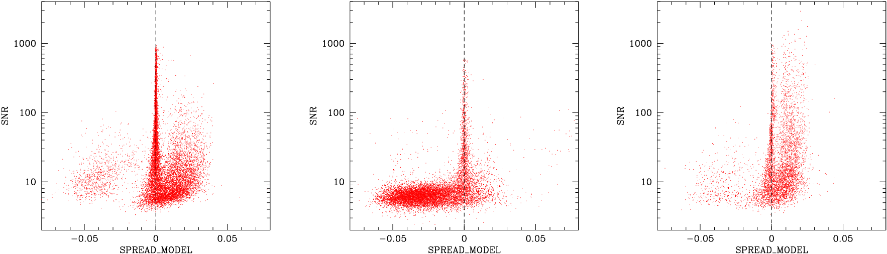
Fig. 10 SNR vs SPREAD_MODEL for three exposures from [27]. Left plot: “good” exposure; extended sources (galaxies and nebulous features) are on the right handside of the stellar locus, and electronic glitches create a small cloud of points on the left handside. Middle: exposure with an unusual amount of electronic glitches. Right: exposure with tracking/guiding issues; the PSF is too complex for individual sources to be identified as a single objects.
The pdf of SPREAD_MODEL is close to Gaussian for isolated point sources at a given SNR; it gets larger for the fainter sources because of image noise. In order to maintain a certain level of purity or completeness across the whole magnitude range, it is therefore necessary to take into account the uncertainty on SPREAD_MODEL, which can be estimated by propagating the uncertainties on individual pixel values:
where \({\bf V}\) is the noise covariance matrix, which we assume to be diagonal. In practice, one may for instance adopt a threshold for star-galaxy separation which is a combination of a fixed and a variable components, such as \(\sqrt{\epsilon^2 + (\kappa \times {\tt SPREADERR\_MODEL})^2}\), with \(\epsilon \approx 5.10^{-3}\) and \(\kappa \approx 4\).